Start by reading the default report. Use more specific queries only when you need a different effect, reporting scale or confidence level.
The example below is the parallel mediation model from Get started.
Example setup
Read the default report
print(result)
#> wsMed analysis
#> Model: P | DE | Observations: 100
#> Effects:
#> wsMed all | raw scale | mc
#> 95% percentile intervals; 20000 joint draws; SE from effect draws
#> Condition contrast: C2 - C1
#>                                        Estimate Std. Error  CI lower  CI upper
#> cp: Direct effect                     -0.031795   0.017000 -0.064525  0.001864
#> indirect_1: M1                         0.001311   0.003208 -0.004586  0.008760
#> indirect_2: M2                        -0.001120   0.002587 -0.007507  0.003186
#> total_indirect: Total indirect effect  0.000191   0.004138 -0.008459  0.008723
#> total: Total effect                   -0.031604   0.017049 -0.064633  0.001895
#> Inference draws: 20000 retained of 20000 ; 0 excluded before effect extraction.
#> Use as.data.frame() for the full-precision table and metadata.
#> Post-fit admissibility: 1 of 1 ; excluded rows: 0
print() displays the core effects and analysis
information. The report gives the estimate, SE and CI for each specific
indirect effect, the total indirect effect, the direct effect and the
total effect. Here the default output is unstandardized, with 95% Monte
Carlo CIs.
Get a statistical summary
summary(result)
#> wsMed statistical summary
#> Model: P | Missing: DE | Observations: 100
#> Effects:
#> wsMed all | raw scale | mc
#> 95% percentile intervals; 20000 joint draws; SE from effect draws
#> Condition contrast: C2 - C1
#>                                        Estimate Std. Error  CI lower  CI upper
#> cp: Direct effect                     -0.031795   0.017000 -0.064525  0.001864
#> indirect_1: M1                         0.001311   0.003208 -0.004586  0.008760
#> indirect_2: M2                        -0.001120   0.002587 -0.007507  0.003186
#> total_indirect: Total indirect effect  0.000191   0.004138 -0.008459  0.008723
#> total: Total effect                   -0.031604   0.017049 -0.064633  0.001895
#> Inference draws: 20000 retained of 20000 ; 0 excluded before effect extraction.
#> Use as.data.frame() for the full-precision table and metadata.
#>
#> Path coefficients:
#>    Estimate Std. Error CI lower CI upper
#> cp -0.03180    0.01700 -0.06453  0.00186
#> b1 -0.04834    0.09555 -0.23422  0.13918
#> d1 -0.06905    0.09524 -0.25390  0.11568
#> b2 -0.07732    0.09387 -0.26459  0.10461
#> d2 -0.03676    0.08675 -0.20684  0.13625
#> a1 -0.02712    0.01772 -0.06162  0.00817
#> a2  0.01448    0.01796 -0.02032  0.04929
#> Post-fit admissibility: 1 of 1 ; excluded rows: 0
#> Tables: $effects, $coefficients; analysis settings: $info.
summary() returns a structured report containing
effects, path coefficients and analysis settings; its default display
shows the statistical tables. Unlike print(), it creates a
summary object that can be saved and reused:
s <- summary(result)Typing s displays the same summary. Neither operation
repeats fitting or sampling. The stored tables retain full precision
even though the printed values are rounded.
Plot the results
plot(result)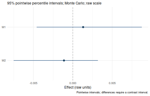
The default plot of this model shows the specific indirect effects.
To plot all effects selected in the summary, use plot(s).
Both inherit the reporting scale saved during the analysis. See the plot gallery for the available displays
and optional settings.
Choose more specific output
Start with the calls above. The following options change one part of the report without fitting again.
Request standardized effects
summary(
  result,
  standardized = TRUE
)
#> wsMed statistical summary
#> Model: P | Missing: DE | Observations: 100
#> Effects:
#> wsMed all | marginal scale | mc
#> 95% percentile intervals; 20000 joint draws; SE from effect draws
#> Condition contrast: C2 - C1
#> Standardization: effect / marginal model-implied SD(D2 - D1); condition contrast is unscaled.
#> Plug-in marginal outcome-difference SD: 0.169239
#> The denominator is not a moderator-specific conditional SD.
#>                                       Estimate Std. Error CI lower CI upper
#> cp: Direct effect                     -0.18787    0.10032 -0.38252  0.01082
#> indirect_1: M1                         0.00775    0.01858 -0.02674  0.05071
#> indirect_2: M2                        -0.00662    0.01496 -0.04331  0.01831
#> total_indirect: Total indirect effect  0.00113    0.02396 -0.04882  0.05067
#> total: Total effect                   -0.18674    0.10061 -0.38051  0.01125
#> Inference draws: 20000 retained of 20000 ; 0 excluded before effect extraction.
#> Use as.data.frame() for the full-precision table and metadata.
#>
#> Path coefficients:
#>    Estimate Std. Error CI lower CI upper
#> cp  -0.1879     0.1003  -0.3825   0.0108
#> b1  -0.0501     0.0970  -0.2352   0.1423
#> d1  -0.0751     0.1013  -0.2707   0.1264
#> b2  -0.0821     0.0975  -0.2715   0.1099
#> d2  -0.0438     0.1012  -0.2393   0.1587
#> a1  -0.1546     0.1028  -0.3594   0.0470
#> a2   0.0806     0.1011  -0.1153   0.2784
#> Post-fit admissibility: 1 of 1 ; excluded rows: 0
#> Tables: $effects, $coefficients; analysis settings: $info.
For complete condition effects, standardization uses the model-implied marginal SD of the outcome difference. See standardized effects for the treatment of paths, interactions and conditional effects.
If the original call used standardized = TRUE, plain
print(result), summary(result) and
plot(result) already use standardized output.
Select an effect family
summary(
  result,
  type = "indirect"
)
#> wsMed statistical summary
#> Model: P | Missing: DE | Observations: 100
#> Effects:
#> wsMed indirect | raw scale | mc
#> 95% percentile intervals; 20000 joint draws; SE from effect draws
#> Condition contrast: C2 - C1
#>                Estimate Std. Error CI lower CI upper
#> indirect_1: M1  0.00131    0.00321 -0.00459  0.00876
#> indirect_2: M2 -0.00112    0.00259 -0.00751  0.00319
#> Inference draws: 20000 retained of 20000 ; 0 excluded before effect extraction.
#> Use as.data.frame() for the full-precision table and metadata.
#>
#> Path coefficients:
#>    Estimate Std. Error CI lower CI upper
#> cp -0.03180    0.01700 -0.06453  0.00186
#> b1 -0.04834    0.09555 -0.23422  0.13918
#> d1 -0.06905    0.09524 -0.25390  0.11568
#> b2 -0.07732    0.09387 -0.26459  0.10461
#> d2 -0.03676    0.08675 -0.20684  0.13625
#> a1 -0.02712    0.01772 -0.06162  0.00817
#> a2  0.01448    0.01796 -0.02032  0.04929
#> Post-fit admissibility: 1 of 1 ; excluded rows: 0
#> Tables: $effects, $coefficients; analysis settings: $info.
Other selections include "direct",
"total_indirect", "total",
"paths" and "parameters". Use
terms only when selecting particular named effects.
Change the confidence level
summary(
  result,
  level = 0.90
)
#> wsMed statistical summary
#> Model: P | Missing: DE | Observations: 100
#> Effects:
#> wsMed all | raw scale | mc
#> 90% percentile intervals; 20000 joint draws; SE from effect draws
#> Condition contrast: C2 - C1
#>                                        Estimate Std. Error  CI lower  CI upper
#> cp: Direct effect                     -0.031795   0.017000 -0.059453 -0.003589
#> indirect_1: M1                         0.001311   0.003208 -0.003348  0.007167
#> indirect_2: M2                        -0.001120   0.002587 -0.005991  0.002170
#> total_indirect: Total indirect effect  0.000191   0.004138 -0.006581  0.006993
#> total: Total effect                   -0.031604   0.017049 -0.059402 -0.003324
#> Inference draws: 20000 retained of 20000 ; 0 excluded before effect extraction.
#> Use as.data.frame() for the full-precision table and metadata.
#>
#> Path coefficients:
#>    Estimate Std. Error CI lower CI upper
#> cp -0.03180    0.01700 -0.05945 -0.00359
#> b1 -0.04834    0.09555 -0.20435  0.10967
#> d1 -0.06905    0.09524 -0.22561  0.08720
#> b2 -0.07732    0.09387 -0.23305  0.07588
#> d2 -0.03676    0.08675 -0.18004  0.10598
#> a1 -0.02712    0.01772 -0.05624  0.00217
#> a2  0.01448    0.01796 -0.01494  0.04405
#> Post-fit admissibility: 1 of 1 ; excluded rows: 0
#> Tables: $effects, $coefficients; analysis settings: $info.
The interval is recalculated from the stored draws. Effect SEs are sample SDs of the joint effect draws, and effect CIs are percentile intervals.
For a model that stored both inference engines, choose
method = "mc" or method = "bootstrap" in
summary(). The default print() reports
both.
Choose moderator values
For moderated mediation, the default report uses the centering
reference for a continuous moderator and all observed levels for a
categorical moderator. Use at to choose raw values or
category labels. For example, after fitting the second Get started
example:
These are conditional effects at specified values, not effects averaged over the moderator distribution.
Compare two pathways
A difference between effects needs its own CI. Use the stored joint draws to form that difference, then print the result directly:
effects <- wsmed_effects(result)
difference <- wsmed_contrasts(
  effects,
  list(B_minus_A = c(indirect_2 = 1, indirect_1 = -1))
)
print(difference)
#> wsMed contrasts | raw scale | mc
#> 95% percentile intervals; 20000 joint draws; SE from effect draws
#> Condition contrast: C2 - C1
#> Contrast direction (signed weights):
#>  B_minus_A: +1 * M2 -1 * M1
#>           Estimate Std. Error CI lower CI upper
#> B_minus_A -0.00243    0.00410 -0.01184  0.00489
#> Inference draws: 20000 retained of 20000 ; 0 excluded before effect extraction.
#> Use as.data.frame() for the full-precision table and metadata.
B_minus_A is the indirect effect through B minus the
effect through A. Do not subtract separate CI endpoints, or infer a
difference simply because only one of the separate intervals excludes
zero.
Extract or export results when needed
Extraction is useful for further calculations or export; it is not required for ordinary reports and plots.
| Task | Call |
|---|---|
| Effects as a data frame | as.data.frame(s) |
| Selected result columns | effect_table[, columns] |
| Effect estimates | coef(s) |
| Effect CIs | confint(s) |
| Covariance of effect draws | vcov(s) |
| Path-coefficient table | s$coefficients |
| Method, scale and confidence level | s$info |
| Sample size of the fitted data | nobs(result) |
The methods on s concern its selected effects. In
contrast, coef(result), vcov(result) and
confint(result) concern primitive model parameters.
To choose which columns to display, list their names in the order you want. For example, keep the effect name, estimate, SE and both CI limits:
effect_table <- as.data.frame(s)
columns <- c(
  "label",
  "estimate",
  "std.error",
  "conf.low",
  "conf.high"
)
effect_table[, columns]
#>                   label      estimate   std.error     conf.low   conf.high
#> 1         Direct effect -0.0317954295 0.016999695 -0.064525050 0.001863738
#> 2                    M1  0.0013113045 0.003208354 -0.004586379 0.008759829
#> 3                    M2 -0.0011199168 0.002587292 -0.007506753 0.003185604
#> 4 Total indirect effect  0.0001913877 0.004138371 -0.008458737 0.008723282
#> 5          Total effect -0.0316040417 0.017049340 -0.064633149 0.001894936
Remove "std.error" from columns to omit
SEs, or remove "conf.low" and "conf.high" to
omit CIs. names(effect_table) lists all available columns;
for moderated mediation, retain moderator and
at to identify the evaluated values or groups. Use
s$coefficients[, columns] for the path-coefficient
table.
To export the same selected columns:
write.csv(
  effect_table[, columns],
  "mediation-effects.csv",
  row.names = FALSE
)

p <- plot(result)
ggplot2::ggsave(
  "mediation-effects.png",
  plot = p,
  width = 7,
  height = 4.5,
  dpi = 300
)
The CSV contains the selected columns at full precision. Use
as.data.frame(s) instead to export the complete effect
table, including analysis settings. Choose your own filenames when
saving results.
Next: customize a plot, or reuse a fit for another inference method.