Reuse a fit: the staged workflow • wsMed

The staged interface separates model specification, fitting, and inference. You can inspect the output after each stage and reuse it in the next one. This guide follows one parallel-mediation example through those three stages, then shows how to read and extract the results. wsMed() remains available for completing the analysis in one call, as shown in Get started.

The workflow at a glance

Stage and call	Returned object	What is available
1. Specify `wsmed_model()`	`model`: a `wsmed_model`	Variable pairs, condition order, mediator structure, covariates and moderator settings.
2. Fit `wsmed_fit(model, data)`	`fit`: a `wsmed_fit`	Fitted parameters and native SEs, prepared data, model syntax, backend fits and diagnostics.
3. Infer `wsmed_infer(fit)`	`inference`: a `wsmed_inference`	The original fit, joint draws, inference settings and draw diagnostics.
4. Read or extract `summary(inference)` or `wsmed_effects(inference)`	A summary or `wsmed_results`	Effect estimates, SEs, CIs, effect draws and reporting settings.

The first three steps create the analysis objects. The fourth uses those objects to produce tables, plots and contrasts; it does not fit or sample again. At each step below, start with the default display and use the extraction examples only when you need the underlying values.

data(example_data)

These simulated data are complete and in wide format, with one row per participant. A1/A2 and B1/B2 are the mediator pairs; D1/D2 are the outcome pair.

1. Specify the model

Use wsmed_model() to describe the analysis before supplying data. Name each pair with the same two conditions. Here, every difference is after minus before. The names A and B identify the mediator roles in paths and output.

model <- wsmed_model(
  outcome = c(before = "D1", after = "D2"),
  mediators = list(
    A = c(before = "A1", after = "A2"),
    B = c(before = "B1", after = "B2")
  )
)
print(model)
#> wsMed model: P 
#> Difference: after - before 
#> Mediators: A, B

Parallel mediation is the default. The main specification arguments are:

Argument	What it specifies
`outcome`	A named pair of outcome columns. Its order defines the condition contrast.
`mediators`	A named list of mediator pairs. Order determines mediator numbering.
`structure`	`"parallel"`, `"serial"`, `"serial_parallel"`, `"parallel_serial"`, or `"custom"`.
`paths`	For custom models, arrows using mediator role names and `Y`, such as `"A -> B"` and `"B -> Y"`.
`covariates`	A list with `between` column names and/or `within` named pairs.
`moderator`	A list specifying the moderator column and the paths with interactions.

What can you inspect now?

specification <- wsmed_inspect(model, "model")
specification$conditions
#> [1] "before" "after"
specification$mediator_names
#> [1] "A" "B"
column_map <- specification$input_vars

Item	Access
Complete specification	`wsmed_inspect(model, "model")`
Condition names and order	`model$conditions`
Mediator role names	`model$mediator_names`
Paired columns and predictor settings	`model$input_vars`
Model-form code and custom edges	`model$form`, `model$paths`

This object contains no observations, fitted estimates or CIs. Model syntax, transformed data and fit diagnostics become available after fitting.

2. Fit the model

Pass the specification and the wide dataset to wsmed_fit():

fit <- wsmed_fit(
  model,
  data = example_data
)
print(fit)
#> wsMed fit: P | DE | 1 fitted dataset(s)
#> Observations: 100 of 100 input rows
#> Converged: 1 of 1 
#> Condition contrast: after - before 
#> Post-fit admissibility: 1 of 1 ; excluded rows: 0

print(fit) reports the sample size, convergence and diagnostic summary. The fitting default is missing = "error", so missing analysis values require an explicit choice of "listwise", "fiml", or "mi". This differs from the listwise-deletion default of wsMed(); it makes no difference for the complete data used here. Missing-data examples appear below.

For the fitted parameter estimates and their native SEs:

fit_summary <- summary(fit)
print(fit_summary)
#> wsMed fitted parameters (DE)
#> Standard errors from fitted parameter covariance; confidence intervals require inference.
#> Condition contrast: after - before 
#> Post-fit admissibility: 1 of 1 ; excluded rows: 0 
#>                 Estimate Std. Error
#> cp             -3.18e-02   1.70e-02
#> b1             -4.83e-02   9.56e-02
#> d1             -6.91e-02   9.52e-02
#> b2             -7.73e-02   9.33e-02
#> d2             -3.68e-02   8.68e-02
#> a1             -2.71e-02   1.75e-02
#> a2              1.45e-02   1.80e-02
#> Ydiff~~Ydiff    2.81e-02   3.97e-03
#> M1diff~~M1diff  3.08e-02   4.35e-03
#> M2diff~~M2diff  3.23e-02   4.56e-03
#> M1avg~~M1avg    3.39e-02   4.79e-03
#> M1avg~~M2avg    1.08e-02   3.87e-03
#> M2avg~~M2avg    4.07e-02   5.76e-03
#> M1avg~1        -2.22e-18   1.84e-02
#> M2avg~1         3.22e-17   2.02e-02

These are the SEM’s fitted parameters, including regression coefficients, intercepts and variances. Their SEs come from the fitted parameter covariance matrix, or Rubin pooling after MI. They are available before simulation.

What can you extract from the fit?

Item	Access	Returned value
Parameter estimates	`coef(fit)`	Named numeric vector.
Parameter estimates and native SEs	`fit_summary$coefficients`	Numeric matrix.
Parameter covariance	`vcov(fit)`	Covariance matrix; Rubin-pooled after MI.
Number of fitted observations	`nobs(fit)`	One count per fitted dataset.
Generated model syntax	`wsmed_inspect(fit, "syntax")`	Character string.
Prepared analysis variables	`wsmed_inspect(fit, "data")`	Data frame of differences, centered averages and other required variables.
Backend models	`wsmed_inspect(fit, "fits")`	List of lavaan fits; one per imputation for MI.
Fit checks and warnings	`wsmed_inspect(fit, "diagnostics")`	Diagnostic list, including a `by_dataset` table.
Recorded fitting information	`wsmed_inspect(fit, "provenance")`	Recorded software and fitting metadata.

For example, save the estimates, covariance and prepared data for further work:

parameter_estimates <- coef(fit)
parameter_covariance <- vcov(fit)
prepared_data <- wsmed_inspect(fit, "data")
nobs(fit)
#> [1] 100
head(prepared_data)
#>         Ydiff     M1diff      M2diff      M1avg       M2avg
#> 1 -0.21677139 -0.1722935  0.16068969 -0.1000090 -0.35166874
#> 2  0.39173048 -0.2088457  0.06815762 -0.3091593 -0.23200291
#> 3  0.37078168 -0.0395939  0.04733066 -0.3458011 -0.20683550
#> 4 -0.09494456 -0.3903959 -0.17175804 -0.1643716  0.01018087
#> 5 -0.10497217  0.2522317 -0.20559112  0.1062956  0.02496926
#> 6 -0.14741498 -0.1956271 -0.04948771  0.1311617  0.21555420

Inspect the generated equations and check the fitted datasets:

cat(wsmed_inspect(fit, "syntax"))
#> Ydiff ~ cp*1 + b1*M1diff + d1*M1avg + b2*M2diff + d2*M2avg
#> M1diff ~ a1*1
#> M2diff ~ a2*1
#> indirect_1 := a1 * b1
#> indirect_2 := a2 * b2
#> total_indirect := indirect_1 + indirect_2
#> total_effect := cp + total_indirect
fit_checks <- wsmed_inspect(fit, "diagnostics")
fit_checks$by_dataset[c("dataset", "n.used", "converged", "admissible", "warnings")]
#>   dataset n.used converged admissible warnings
#> 1       1    100      TRUE       TRUE        0
fit_checks$warnings
#> character(0)

converged records whether estimation converged; admissible records the backend post-fit check. Review warnings and failed checks before proceeding. Convergence alone does not establish that the model or missing-data assumptions are appropriate. For additional backend diagnostics, retrieve the fits with wsmed_inspect(fit, "fits") and inspect the relevant fitted dataset.

You can also obtain effect point estimates before inference:

point_effects <- wsmed_effects(fit)
print(point_effects)
#> wsMed indirect | raw scale | point 
#> Point estimates only; no simulation-based SE or intervals.
#> Condition contrast: after - before 
#>               Estimate
#> indirect_1: A  0.00131
#> indirect_2: B -0.00112
#> Use as.data.frame() for the full-precision table and metadata.

This defaults to the specific indirect effects. No simulation-based effect SEs or CIs are available yet. confint(fit) therefore asks you to run wsmed_infer() first; plot(fit) likewise shows point estimates only.

3. Perform inference

Pass the existing fit to wsmed_infer():

inference <- wsmed_infer(
  fit,
  seed = 123
)
print(inference)
#> wsMed inference: mc | 20000 valid draws of 20000 requested
#> 95% effect intervals: percentile; stored parameter-table convention: percentile
#> Inference draws: 20000 retained of 20000 ; 0 excluded before effect extraction.
#> Use summary() or wsmed_effects() to select effects.

The defaults are Monte Carlo inference, 20,000 draws and 95% CIs. The seed is specified for reproducibility; the staged default is seed = NULL. print(inference) reports the inference method and the number of retained draws. It does not display the effect table; use summary(inference) next.

What can you extract from inference?

Item	Access	Meaning
Original fitted model	`inference$fit`	The `wsmed_fit` supplied to this stage.
Joint draws	`inference$draws`	One draw per row; columns contain parameters and generated effect definitions.
Draw identities	`inference$draw_ids`	Original identities of retained draws.
Method and settings	`inference$method`, `inference$controls`	Draw count, seed, confidence level and other inference controls.
Inference checks	`wsmed_inspect(inference, "diagnostics")`	Requested, retained and invalid draws, plus recorded warnings.
Parameter point estimates	`coef(inference)`	The same fitted parameter estimates as `coef(fit)`.
Empirical parameter covariance	`vcov(inference)`	Covariance of stored draws for the model parameters.
Parameter CIs	`confint(inference)`	Percentile CIs for model parameters.

For a compact view of the stored joint draws:

joint_draws <- inference$draws
dim(joint_draws)
#> [1] 20000    19
head(
  joint_draws[, c("a1", "b1", "indirect_1")],
  n = 3
)
#>               a1          b1   indirect_1
#> [1,] -0.05060167  0.03051865 -0.001544295
#> [2,] -0.04530387 -0.02753059  0.001247242
#> [3,] -0.04276521  0.15272648 -0.006531380
inference_checks <- wsmed_inspect(inference, "diagnostics")
inference_checks[c("requested", "valid", "invalid")]
#> $requested
#> [1] 20000
#> 
#> $valid
#> [1] 20000
#> 
#> $invalid
#> [1] 0

The coefficients within a row belong to the same draw. Keeping that pairing is necessary when forming products or contrasts. Point estimates remain those computed from the fitted model; they are not replaced by averages of the draws. For conditional or standardized effect draws, use the result object in step 4, which applies the requested transformations and records any additional exclusions.

wsmed_inspect(inference, "diagnostics") describes inference. To recover the fitting checks, use wsmed_inspect(inference$fit, "diagnostics").

4. Read and extract effect results

Start with the default statistical summary and plot:

s <- summary(inference)
print(s)
#> wsMed statistical summary
#> Model: P | Missing: DE | Observations: 100 
#> Effects:
#> wsMed all | raw scale | mc 
#> 95% percentile intervals; 20000 joint draws; SE from effect draws
#> Condition contrast: after - before 
#>                                        Estimate Std. Error  CI lower  CI upper
#> cp: Direct effect                     -0.031795   0.017000 -0.064525  0.001864
#> indirect_1: A                          0.001311   0.003208 -0.004586  0.008760
#> indirect_2: B                         -0.001120   0.002587 -0.007507  0.003186
#> total_indirect: Total indirect effect  0.000191   0.004138 -0.008459  0.008723
#> total: Total effect                   -0.031604   0.017049 -0.064633  0.001895
#> Inference draws: 20000 retained of 20000 ; 0 excluded before effect extraction.
#> Use as.data.frame() for the full-precision table and metadata.
#> 
#> Path coefficients:
#>    Estimate Std. Error CI lower CI upper
#> cp -0.03180    0.01700 -0.06453  0.00186
#> b1 -0.04834    0.09555 -0.23422  0.13918
#> d1 -0.06905    0.09524 -0.25390  0.11568
#> b2 -0.07732    0.09387 -0.26459  0.10461
#> d2 -0.03676    0.08675 -0.20684  0.13625
#> a1 -0.02712    0.01772 -0.06162  0.00817
#> a2  0.01448    0.01796 -0.02032  0.04929
#> Post-fit admissibility: 1 of 1 ; excluded rows: 0 
#> Tables: $effects, $coefficients; analysis settings: $info.

plot(inference)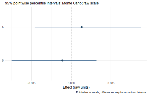

plot of chunk default-plot

The summary displays the direct effect, specific indirect effects, total indirect effect and total effect, followed by path coefficients. The default plot displays the specific indirect effects. Each effect SE is the sample SD of its draws, and its CI is a percentile interval from those draws.

What can you extract from the summary?

Item	Access
Effect table: estimates, SEs, CIs and metadata	`s$effects` or `as.data.frame(s)`
Path-coefficient table	`s$coefficients`
Reporting settings: method, scale, confidence level and probes	`s$info`
Selected effect estimates	`coef(s)`
Selected effect CIs	`confint(s)`
Covariance of selected effect draws	`vcov(s)`
Joint draws for the selected effects	`s$draws`
Draw identities and effect-level exclusions	`s$draw_ids`, `s$diagnostics`
Fitting diagnostics retained in the summary	`s$fit_diagnostics`

For example, retain just the effect name, estimate, SE and CI columns:

effect_table <- as.data.frame(s)
columns <- c(
  "label",
  "estimate",
  "std.error",
  "conf.low",
  "conf.high"
)
effect_table[, columns]
#>                   label      estimate   std.error     conf.low   conf.high
#> 1         Direct effect -0.0317954295 0.016999695 -0.064525050 0.001863738
#> 2                     A  0.0013113045 0.003208354 -0.004586379 0.008759829
#> 3                     B -0.0011199168 0.002587292 -0.007506753 0.003185604
#> 4 Total indirect effect  0.0001913877 0.004138371 -0.008458737 0.008723282
#> 5          Total effect -0.0316040417 0.017049340 -0.064633149 0.001894936

Remove names from columns to omit them, or reorder them to change the display. The same selection works on s$coefficients. Tables retain full precision; the digits argument to print() changes only the display.

The object passed to an accessor determines what it returns:

Call	Quantity
`coef(fit)` or `coef(inference)`	Fitted SEM parameters.
`vcov(fit)`	Native fitted parameter covariance.
`vcov(inference)`	Empirical covariance of model-parameter draws.
`confint(inference)`	CIs for model parameters.
`coef(s)`, `vcov(s)`, `confint(s)`	Estimates, draw covariance and CIs for the effects selected in the summary.

For indirect-effect CIs, use a summary or an effect result object, rather than confint(inference). For example:

effects <- wsmed_effects(inference)
print(effects)
#> wsMed indirect | raw scale | mc 
#> 95% percentile intervals; 20000 joint draws; SE from effect draws
#> Condition contrast: after - before 
#>               Estimate Std. Error CI lower CI upper
#> indirect_1: A  0.00131    0.00321 -0.00459  0.00876
#> indirect_2: B -0.00112    0.00259 -0.00751  0.00319
#> Inference draws: 20000 retained of 20000 ; 0 excluded before effect extraction.
#> Use as.data.frame() for the full-precision table and metadata.
confint(effects)
#>                   2.5 %      97.5 %
#> indirect_1 -0.004586379 0.008759829
#> indirect_2 -0.007506753 0.003185604

wsmed_effects() defaults to specific indirect effects. Its wsmed_results object stores $table, $point, $draws, $draw_ids, $query, and $diagnostics. $query records the requested effect family, reporting scale, moderator values and confidence level. In contrast, summary() defaults to all core effects and adds the path-coefficient table and $info.

To compare the two indirect effects, use the same joint draws:

contrast <- wsmed_contrasts(
  effects,
  list(B_minus_A = c(indirect_2 = 1, indirect_1 = -1))
)
print(contrast)
#> wsMed contrasts | raw scale | mc 
#> 95% percentile intervals; 20000 joint draws; SE from effect draws
#> Condition contrast: after - before 
#> Contrast direction (signed weights):
#>  B_minus_A: +1 * B -1 * A
#>           Estimate Std. Error CI lower CI upper
#> B_minus_A -0.00243    0.00410 -0.01184  0.00489
#> Inference draws: 20000 retained of 20000 ; 0 excluded before effect extraction.
#> Use as.data.frame() for the full-precision table and metadata.

The contrast CI comes from the draw-by-draw difference, not from subtracting the endpoints of two separate CIs. See Read and export results for further selection and export examples.

Decide where to restart after a change

What changed?	Where to continue
Variable roles, mediator structure, covariates or moderated paths	Specify a new model, then fit and infer.
Dataset, missing-data strategy or imputation settings	Run `wsmed_fit()` with the relevant model, then infer.
Monte Carlo versus bootstrap, number of draws, or inference seed	Run `wsmed_infer()` on the existing fit.
Selected effects, moderator probes, confidence level or reporting scale	Query the existing inference or result object.
Labels, rounding or plot appearance	Reprint or replot existing results.

For example, the following queries reuse the same inference draws:

summary(
  effects,
  level = 0.90
)
#> wsMed indirect | raw scale | mc 
#> 90% percentile intervals; 20000 joint draws; SE from effect draws
#> Condition contrast: after - before 
#>               Estimate Std. Error CI lower CI upper
#> indirect_1: A  0.00131    0.00321 -0.00335  0.00717
#> indirect_2: B -0.00112    0.00259 -0.00599  0.00217
#> Inference draws: 20000 retained of 20000 ; 0 excluded before effect extraction.
#> Use as.data.frame() for the full-precision table and metadata.
summary(
  inference,
  standardized = TRUE
)
#> wsMed statistical summary
#> Model: P | Missing: DE | Observations: 100 
#> Effects:
#> wsMed all | marginal scale | mc 
#> 95% percentile intervals; 20000 joint draws; SE from effect draws
#> Condition contrast: after - before 
#> Standardization: effect / marginal model-implied SD(D2 - D1); condition contrast is unscaled.
#> Plug-in marginal outcome-difference SD: 0.169239 
#> The denominator is not a moderator-specific conditional SD.
#>                                       Estimate Std. Error CI lower CI upper
#> cp: Direct effect                     -0.18787    0.10032 -0.38252  0.01082
#> indirect_1: A                          0.00775    0.01858 -0.02674  0.05071
#> indirect_2: B                         -0.00662    0.01496 -0.04331  0.01831
#> total_indirect: Total indirect effect  0.00113    0.02396 -0.04882  0.05067
#> total: Total effect                   -0.18674    0.10061 -0.38051  0.01125
#> Inference draws: 20000 retained of 20000 ; 0 excluded before effect extraction.
#> Use as.data.frame() for the full-precision table and metadata.
#> 
#> Path coefficients:
#>    Estimate Std. Error CI lower CI upper
#> cp  -0.1879     0.1003  -0.3825   0.0108
#> b1  -0.0501     0.0970  -0.2352   0.1423
#> d1  -0.0751     0.1013  -0.2707   0.1264
#> b2  -0.0821     0.0975  -0.2715   0.1099
#> d2  -0.0438     0.1012  -0.2393   0.1587
#> a1  -0.1546     0.1028  -0.3594   0.0470
#> a2   0.0806     0.1011  -0.1153   0.2784
#> Post-fit admissibility: 1 of 1 ; excluded rows: 0 
#> Tables: $effects, $coefficients; analysis settings: $info.

Alternatively, set standardized = TRUE in wsmed_fit() to save standardized reporting as the default. This does not change model fitting. Standardized effects use the model-implied scales and propagate their uncertainty across the joint draws; see standardized effects.

To create a separate bootstrap inference from the same fit:

bootstrap_inference <- wsmed_infer(
  fit,
  method = "bootstrap",
  seed = 123
)
summary(bootstrap_inference)

This uses the default 2,000 bootstrap replicates. Bootstrap necessarily fits the resampled datasets; it retains the original fitted object. The interval argument controls the stored legacy parameter table. Effect and confint() methods use percentile intervals, including when that parameter table uses a bias-corrected convention.

Add a custom structure and moderator

Changes to the model belong in step 1. In the staged interface, custom arrows and moderated slopes use the mediator role names, rather than the M1/M2 and MP labels used by wsMed(). The following model has A to C, C to the outcome, and B to the outcome, with moderation of the first two slopes:

moderated_model <- wsmed_model(
  outcome = c(before = "D1", after = "D2"),
  mediators = list(
    A = c(before = "A1", after = "A2"),
    B = c(before = "B1", after = "B2"),
    C = c(before = "C1", after = "C2")
  ),
  structure = "custom",
  paths = c("A -> C", "C -> Y", "B -> Y"),
  moderator = list(
    variable = "D3",
    interactions = c("A -> C", "C -> Y")
  )
)
mod_fit <- wsmed_fit(
  moderated_model,
  data = example_data
)
mod_inference <- wsmed_infer(
  mod_fit,
  seed = 123
)
summary(mod_inference)
#> wsMed statistical summary
#> Model: UD | Missing: DE | Observations: 100 
#> Effects:
#> wsMed all | raw scale | mc 
#> 95% percentile intervals; 20000 joint draws; SE from effect draws
#> Condition contrast: after - before 
#> Moderator: D3 in raw units; centering reference = 0.452271 
#>                                                       Estimate Std. Error
#> cp@1: Direct effect [D3 = 0.452]                     -0.029850   0.016991
#> indirect_1_3@1: A -> C [D3 = 0.452]                  -0.000022   0.000367
#> indirect_2@1: B [D3 = 0.452]                         -0.001400   0.002744
#> indirect_3@1: C [D3 = 0.452]                         -0.000183   0.002168
#> total_indirect@1: Total indirect effect [D3 = 0.452] -0.001605   0.003581
#> total@1: Total effect [D3 = 0.452]                   -0.031455   0.017152
#>                                                       CI lower  CI upper
#> cp@1: Direct effect [D3 = 0.452]                     -0.063464  0.003219
#> indirect_1_3@1: A -> C [D3 = 0.452]                  -0.000838  0.000719
#> indirect_2@1: B [D3 = 0.452]                         -0.008152  0.003015
#> indirect_3@1: C [D3 = 0.452]                         -0.005150  0.004257
#> total_indirect@1: Total indirect effect [D3 = 0.452] -0.009945  0.004960
#> total@1: Total effect [D3 = 0.452]                   -0.065383  0.002083
#> Inference draws: 20000 retained of 20000 ; 0 excluded before effect extraction.
#> Use as.data.frame() for the full-precision table and metadata.
#> 
#> Path coefficients:
#>                             Estimate Std. Error CI lower CI upper
#> cp@1: cp [D3 = 0.452]       -0.02985    0.01699 -0.06346  0.00322
#> b2@1: b2 [D3 = 0.452]       -0.09668    0.09286 -0.27706  0.08467
#> d2@1: d2 [D3 = 0.452]       -0.00641    0.08965 -0.18213  0.16843
#> b3@1: b3 [D3 = 0.452]       -0.01370    0.10379 -0.21420  0.19224
#> d3@1: d3 [D3 = 0.452]       -0.15680    0.10278 -0.35544  0.04381
#> a1@1: a1 [D3 = 0.452]       -0.02712    0.01728 -0.06113  0.00670
#> a2@1: a2 [D3 = 0.452]        0.01448    0.01791 -0.02029  0.04996
#> a3@1: a3 [D3 = 0.452]        0.01336    0.01623 -0.01834  0.04508
#> b_1_3@1: b_1_3 [D3 = 0.452] -0.05915    0.09216 -0.24131  0.12014
#> d_1_3@1: d_1_3 [D3 = 0.452] -0.05761    0.09046 -0.23376  0.11900
#> Post-fit admissibility: 1 of 1 ; excluded rows: 0 
#> Tables: $effects, $coefficients; analysis settings: $info.

interactions selects difference-component slopes. To moderate an average-component slope, use average_interactions in the moderator list. Moderator main effects enter all difference equations by default. This example corresponds to form = "UD" with paths = c("M1 -> M3", "M3 -> Y", "M2 -> Y") and MP = c("b_1_3", "b3") in the one-call UD tutorial.

The same extraction functions remain available at each stage. For example, wsmed_inspect(mod_fit, "syntax") shows the fitted interaction terms, and summary(mod_inference)$coefficients contains conditional path coefficients. The default continuous-moderator summary uses the centering reference shown in the output; the default plot displays indirect effects across its range:

plot(mod_inference)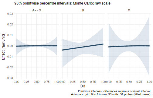

plot of chunk moderated-plot

To choose raw moderator values and retain a conditional-effect table:

conditional <- wsmed_effects(
  mod_inference,
  at = list(D3 = c(0.2, 0.4, 0.6))
)
print(conditional)
#> wsMed indirect | raw scale | mc 
#> 95% percentile intervals; 20000 joint draws; SE from effect draws
#> Condition contrast: after - before 
#> Moderator: D3 in raw units; centering reference = 0.452271 
#>                                    Estimate Std. Error  CI lower  CI upper
#> indirect_1_3@1: A -> C [D3 = 0.2] -1.21e-04   1.25e-03 -2.92e-03  2.38e-03
#> indirect_2@1: B [D3 = 0.2]        -2.79e-03   4.45e-03 -1.38e-02  4.15e-03
#> indirect_3@1: C [D3 = 0.2]        -5.60e-04   4.85e-03 -1.15e-02  9.48e-03
#> indirect_1_3@2: A -> C [D3 = 0.4] -3.54e-05   4.23e-04 -9.91e-04  8.10e-04
#> indirect_2@2: B [D3 = 0.4]        -1.69e-03   2.94e-03 -8.96e-03  2.92e-03
#> indirect_3@2: C [D3 = 0.4]        -2.44e-04   2.33e-03 -5.57e-03  4.56e-03
#> indirect_1_3@3: A -> C [D3 = 0.6] -3.81e-07   4.78e-04 -9.97e-04  1.03e-03
#> indirect_2@3: B [D3 = 0.6]        -5.86e-04   2.90e-03 -7.41e-03  5.16e-03
#> indirect_3@3: C [D3 = 0.6]        -5.77e-05   2.74e-03 -6.19e-03  5.82e-03
#> Inference draws: 20000 retained of 20000 ; 0 excluded before effect extraction.
#> Use as.data.frame() for the full-precision table and metadata.

conditional$table contains the estimates and CIs at those values; conditional$draws contains the corresponding joint effect draws. Supply raw values even when requesting standardized output. Invalid standardized draws are excluded jointly, with original identities recorded in $diagnostics$invalid_draw_ids. Plot bands are pointwise, not simultaneous.

For categorical covariates and moderators, use unordered factors with explicit levels; the first level is the reference group. Numeric 0/1 columns remain continuous in the staged interface unless converted to factors. Default categorical probes include all observed levels. See categorical predictors for coding and group contrasts.

Handle missing data at the fitting stage

The model specification can be reused with incomplete data. To demonstrate, remove a few measurements from a copy of the simulated data:

incomplete_data <- example_data
incomplete_data$A2[1:5] <- NA
incomplete_data$D2[6:10] <- NA

`missing`	What fitting does	Inference methods
`"error"` (default)	Requires complete analysis variables.	Monte Carlo or bootstrap.
`"listwise"`	Uses complete cases for the analysis variables.	Monte Carlo or bootstrap.
`"fiml"`	Handles missing analysis variables during model fitting.	Monte Carlo or bootstrap.
`"mi"`	Imputes original measurements, constructs variables within each completed dataset, fits and pools.	Monte Carlo only.

For FIML, use wsmed_fit(model, incomplete_data, missing = "fiml"). Categorical predictors must be fully observed under FIML. For MI, set its controls at fitting and the inference seed separately:

mi_fit <- wsmed_fit(
  model,
  data = incomplete_data,
  missing = "mi",
  mi = list(seed = 123)
)
mi_inference <- wsmed_infer(
  mi_fit,
  seed = 604
)
print(mi_fit)
#> wsMed fit: P | MI | 5 fitted dataset(s)
#> Observations: 100 of 100 input rows
#> Converged: 5 of 5 
#> Condition contrast: after - before 
#> MI: per-imputation centering; first-imputation reporting reference.
#> Post-fit admissibility: 5 of 5 ; excluded rows: 0
print(mi_inference)
#> wsMed inference: mc | 20000 valid draws of 20000 requested
#> 95% effect intervals: percentile; stored parameter-table convention: percentile
#> Inference draws: 20000 retained of 20000 ; 0 excluded before effect extraction.
#> Use summary() or wsmed_effects() to select effects.

This uses the default five imputations and numeric imputation method. Choose appropriate settings for an actual analysis; for example, mi = list(m = 20, method = "pmm", seed = 123) explicitly requests 20 predictive-mean-matching imputations. A new wsmed_infer(mi_fit, ...) call reuses the fitted imputations and pooled quantities without reimputing.

What changes in extraction after MI?

Item	Access
Pooled parameter estimates and total covariance	`coef(mi_fit)`, `vcov(mi_fit)`
All backend fits	`wsmed_inspect(mi_fit, "fits")`
Counts and checks for every imputation	`nobs(mi_fit)`, `wsmed_inspect(mi_fit, "diagnostics")$by_dataset`
Prepared data for the first imputation	`wsmed_inspect(mi_fit, "data")`
Prepared data for all imputations	`mi_fit$mi$prepared$processed_data_list`
Pooled effect summaries and their draws	`summary(mi_inference)`, `wsmed_effects(mi_inference)`

For example, retrieve the fitted models and transformed datasets:

imputation_fits <- wsmed_inspect(mi_fit, "fits")
prepared_imputations <- mi_fit$mi$prepared$processed_data_list
length(imputation_fits)
#> [1] 5
length(prepared_imputations)
#> [1] 5
nobs(mi_fit)
#> [1] 100 100 100 100 100

wsmed_inspect(mi_fit, "data") returns one data frame, not the complete list of imputations. Do not use the first imputation’s backend fit as a substitute for pooled inference. The workflow retains per-imputation centering and the first-imputation moderator reference for reporting.

For externally generated imputations, pass mi = list(completed = completed) with missing = "mi". completed can be a list of completed wide datasets or a mice mids object. Their number is inferred; omit internal imputation-method and seed controls. With moderation, default main-effects imputation may not preserve the specified interactions. See model-compatible imputation for choosing and supplying an appropriate imputation model.

Relate the stages to a one-call analysis

For the original complete-data example, the equivalent one-call analysis is:

result <- wsMed(
  data = example_data,
  M_C1 = c("A1", "B1"),
  M_C2 = c("A2", "B2"),
  Y_C1 = "D1",
  Y_C2 = "D2"
)
print(result)
#> wsMed analysis
#> Model: P | DE | Observations: 100 
#> Effects:
#> wsMed all | raw scale | mc 
#> 95% percentile intervals; 20000 joint draws; SE from effect draws
#> Condition contrast: C2 - C1 
#>                                        Estimate Std. Error  CI lower  CI upper
#> cp: Direct effect                     -0.031795   0.017000 -0.064525  0.001864
#> indirect_1: M1                         0.001311   0.003208 -0.004586  0.008760
#> indirect_2: M2                        -0.001120   0.002587 -0.007507  0.003186
#> total_indirect: Total indirect effect  0.000191   0.004138 -0.008459  0.008723
#> total: Total effect                   -0.031604   0.017049 -0.064633  0.001895
#> Inference draws: 20000 retained of 20000 ; 0 excluded before effect extraction.
#> Use as.data.frame() for the full-precision table and metadata.
#> Post-fit admissibility: 1 of 1 ; excluded rows: 0

Both analyses use 20,000 Monte Carlo draws and seed 123. The variable roles are named differently in the displays, but the numerical effects and draws match in this example. wsMed() uses the same fitting and inference engines. With missing data, align the missing-data strategy as well as the inference settings before comparing the interfaces.

Save a stage and continue later

Save the inference object to retain both its fit and its draws:

saveRDS(
  inference,
  "mediation-inference.rds"
)
restored <- readRDS("mediation-inference.rds")
summary(restored)

Saving fit instead retains the fitted model for a later wsmed_infer() call. An analysis manifest records settings, diagnostics and software versions:

manifest <- wsmed_reproducibility(inference)
names(manifest)
#> [1] "report_schema_version" "model"                 "analysis"             
#> [4] "fitting_versions"      "fit_diagnostics"       "inference"            
#> [7] "export_environment"

The manifest does not contain observations or draws and does not replace the saved object, data and analysis script. Seeded workflow calls restore the caller’s random state; seed = NULL advances the current random stream. For older saved objects, compatibility checks may require refitting or regenerating inference; the accessors do not silently reconstruct missing metadata. See diagnostics and migration.