Standardized effects
Source:vignettes/StandardizedModeratedMediation.Rmd
StandardizedModeratedMediation.RmdRequest standardized results
Standardization is available with or without a
moderator. Set standardized = TRUE in the
analysis; subsequent summaries and generic plots inherit that
preference.
data(example_data)
standardized_intro <- wsMed(
  example_data,
  M_C1 = c("A1", "B1"),
  M_C2 = c("A2", "B2"),
  Y_C1 = "D1",
  Y_C2 = "D2",
  standardized = TRUE
)
print(standardized_intro)
#> wsMed analysis
#> Model: P | DE | Observations: 100
#> Effects:
#> wsMed all | marginal scale | mc
#> 95% percentile intervals; 20000 joint draws; SE from effect draws
#> Condition contrast: C2 - C1
#> Standardization: effect / marginal model-implied SD(D2 - D1); condition contrast is unscaled.
#> Plug-in marginal outcome-difference SD: 0.169239
#> The denominator is not a moderator-specific conditional SD.
#>                                       Estimate Std. Error CI lower CI upper
#> cp: Direct effect                     -0.18787    0.10032 -0.38252  0.01082
#> indirect_1: M1                         0.00775    0.01858 -0.02674  0.05071
#> indirect_2: M2                        -0.00662    0.01496 -0.04331  0.01831
#> total_indirect: Total indirect effect  0.00113    0.02396 -0.04882  0.05067
#> total: Total effect                   -0.18674    0.10061 -0.38051  0.01125
#> Inference draws: 20000 retained of 20000 ; 0 excluded before effect extraction.
#> Use as.data.frame() for the full-precision table and metadata.
#> Post-fit admissibility: 1 of 1 ; excluded rows: 0
These complete condition effects are expressed relative to the
marginal SD of the outcome difference. For a one-off unstandardized
query, use
summary(standardized_intro, standardized = FALSE). See the
results guide for table export.
Choose what to read next: definitions, continuous moderators, categorical moderators, or missing data.
What is standardized?
For a two-condition design, define
and
.
PrepareData() centers the mediator average component, but
does not center these differences. Standardization divides a difference
by its marginal model-implied SD, preserving its mean condition
effect.
Write and . Without moderation,
The condition contrast retains its original unit. In a serial chain, the intermediate mediator SDs cancel. Thus every complete indirect effect, its contrast with another complete indirect effect, the total indirect effect and the total condition effect use the outcome-difference SD.
These are marginal SDs implied by the fitted model, not residual SDs, group-specific SDs or SDs conditional on a selected moderator value. The same endpoint scales apply at every moderator value within a fit.
Continuous moderators: two different quantities
For a centered moderator , suppose the conditional paths are and . Then
The standardized interaction coefficient is instead
Standardized interaction coefficients are expressed per SD of a
continuous moderator. In contrast, summary(result) reports
conditional effects and paths at selected raw moderator values.
Conditional tables and curves evaluate effects at fixed numerical
moderator values in the original units. To recover a
conditional slope from fully standardized coefficients, use
.
The scale of an interaction is the product of its component scale
factors, not the SD of the observed product column.
Fit a reproducible example
The following simulated data have a moderator with a nonzero mean and an SD different from one. The mediator averages and differences are generated separately to make the two-condition structure explicit.
set.seed(918)
n <- 350
w <- rnorm(n, 3, 2)
avg1 <- rnorm(n)
avg2 <- rnorm(n)
dm1 <- 2 + 0.8 * w + rnorm(n)
dm2 <- 1 + 0.4 * w + 0.3 * dm1 + rnorm(n)
dy <- 0.5 + 0.6 * w + 0.5 * dm1 + 0.7 * dm2 +
      0.2 * dm1 * w + 0.3 * avg1 + rnorm(n)
y1 <- rnorm(n)
dat <- data.frame(
  M11 = avg1 - dm1/2,
  M12 = avg1 + dm1/2,
  M21 = avg2 - dm2/2,
  M22 = avg2 + dm2/2,
  Y1 = y1,
  Y2 = y1 + dy,
  W = w
)
result <- wsMed(
  data = dat,
  M_C1 = c("M11", "M21"),
  M_C2 = c("M12", "M22"),
  Y_C1 = "Y1",
  Y_C2 = "Y2",
  W = "W",
  MP = c("b1", "d1"),
  standardized = TRUE
)
print(result)
#> wsMed analysis
#> Model: P | DE | Observations: 350
#> Effects:
#> wsMed all | marginal scale | mc
#> 95% percentile intervals; 20000 joint draws; SE from effect draws
#> Condition contrast: C2 - C1
#> Moderator: W in raw units; centering reference = 3.23288
#> Standardization: effect / marginal model-implied SD(Y2 - Y1); condition contrast is unscaled.
#> Plug-in marginal outcome-difference SD: 6.28886
#> The denominator is not a moderator-specific conditional SD.
#>                                                    Estimate Std. Error CI lower
#> cp@1: Direct effect [W = 3.23]                       0.3392     0.0535   0.2375
#> indirect_1@1: M1 [W = 3.23]                          0.8545     0.0510   0.7597
#> indirect_2@1: M2 [W = 3.23]                          0.4512     0.0364   0.3818
#> total_indirect@1: Total indirect effect [W = 3.23]   1.3057     0.0705   1.1741
#> total@1: Total effect [W = 3.23]                     1.6449     0.0650   1.5285
#>                                                    CI upper
#> cp@1: Direct effect [W = 3.23]                       0.4477
#> indirect_1@1: M1 [W = 3.23]                          0.9590
#> indirect_2@1: M2 [W = 3.23]                          0.5243
#> total_indirect@1: Total indirect effect [W = 3.23]   1.4527
#> total@1: Total effect [W = 3.23]                     1.7822
#> Inference draws: 20000 retained of 20000 ; 0 excluded before effect extraction.
#> Use as.data.frame() for the full-precision table and metadata.
#> Post-fit admissibility: 1 of 1 ; excluded rows: 0
summary(result)
#> wsMed statistical summary
#> Model: P | Missing: DE | Observations: 350
#> Effects:
#> wsMed all | marginal scale | mc
#> 95% percentile intervals; 20000 joint draws; SE from effect draws
#> Condition contrast: C2 - C1
#> Moderator: W in raw units; centering reference = 3.23288
#> Standardization: effect / marginal model-implied SD(Y2 - Y1); condition contrast is unscaled.
#> Plug-in marginal outcome-difference SD: 6.28886
#> The denominator is not a moderator-specific conditional SD.
#>                                                    Estimate Std. Error CI lower
#> cp@1: Direct effect [W = 3.23]                       0.3392     0.0535   0.2375
#> indirect_1@1: M1 [W = 3.23]                          0.8545     0.0510   0.7597
#> indirect_2@1: M2 [W = 3.23]                          0.4512     0.0364   0.3818
#> total_indirect@1: Total indirect effect [W = 3.23]   1.3057     0.0705   1.1741
#> total@1: Total effect [W = 3.23]                     1.6449     0.0650   1.5285
#>                                                    CI upper
#> cp@1: Direct effect [W = 3.23]                       0.4477
#> indirect_1@1: M1 [W = 3.23]                          0.9590
#> indirect_2@1: M2 [W = 3.23]                          0.5243
#> total_indirect@1: Total indirect effect [W = 3.23]   1.4527
#> total@1: Total effect [W = 3.23]                     1.7822
#> Inference draws: 20000 retained of 20000 ; 0 excluded before effect extraction.
#> Use as.data.frame() for the full-precision table and metadata.
#>
#> Path coefficients:
#>                      Estimate Std. Error  CI lower  CI upper
#> cp@1: cp [W = 3.23]  0.339206   0.053507  0.237543  0.447743
#> b1@1: b1 [W = 3.23]  0.352858   0.017579  0.318425  0.387543
#> d1@1: d1 [W = 3.23]  0.037421   0.008851  0.020355  0.055020
#> b2@1: b2 [W = 3.23]  0.209823   0.015722  0.179426  0.240768
#> d2@1: d2 [W = 3.23] -0.000698   0.008546 -0.017691  0.015856
#> a1@1: a1 [W = 3.23]  2.421621   0.095983  2.245296  2.618727
#> a2@1: a2 [W = 3.23]  2.150475   0.087890  1.988346  2.333949
#> Post-fit admissibility: 1 of 1 ; excluded rows: 0
#> Tables: $effects, $coefficients; analysis settings: $info.
MP requests interactions and focal paths. Moderator main
effects already included in the fitted regressions also enter
conditional intercepts, even when a1 or cp is
absent from MP. The total indirect effect includes both
mediator paths in this example, not just the path with a requested
interaction.
The default report and summary inherit
standardized = TRUE. Use
summary(result, standardized = FALSE) to request
unstandardized results without fitting again. Use
wsmed_effects(result) when you need a separate effect table
for further comparisons or export.
plot(result)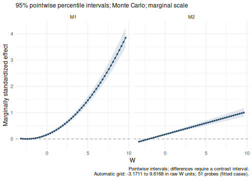
The horizontal axis retains raw moderator units. The default curves show specific indirect effects with pointwise CIs over the observed range. They are not simultaneous confidence bands or exact Johnson–Neyman regions.
Categorical moderators
Categorical moderators retain their 0/1 dummy coding. There is no SD-of-dummy multiplier, and all groups share the same marginal endpoint scales. The factor levels below make the reference category explicit.
dat$Group <- cut(dat$W, c(-Inf, 2, 4, Inf), labels = c("A", "B", "C"))
levels(dat$Group)
#> [1] "A" "B" "C"
group_result <- wsMed(
  data = dat,
  M_C1 = c("M11", "M21"),
  M_C2 = c("M12", "M22"),
  Y_C1 = "Y1",
  Y_C2 = "Y2",
  W = "Group",
  MP = c("b1", "d1"),
  standardized = TRUE
)
print(group_result)
#> wsMed analysis
#> Model: P | DE | Observations: 350
#> Effects:
#> wsMed all | marginal scale | mc
#> 95% percentile intervals; 20000 joint draws; SE from effect draws
#> Condition contrast: C2 - C1
#> Moderator: Group ; reference category = A
#> Standardization: effect / marginal model-implied SD(Y2 - Y1); condition contrast is unscaled.
#> Plug-in marginal outcome-difference SD: 6.05489
#> The denominator is not a moderator-specific conditional SD.
#>                                                     Estimate Std. Error
#> cp@1: Direct effect [Group = A]                      -0.0196     0.0649
#> indirect_1@1: M1 [Group = A]                          0.4185     0.0612
#> indirect_2@1: M2 [Group = A]                          0.4019     0.0365
#> total_indirect@1: Total indirect effect [Group = A]   0.8204     0.0757
#> total@1: Total effect [Group = A]                     0.8008     0.0559
#> cp@2: Direct effect [Group = B]                       0.0997     0.0939
#> indirect_1@2: M1 [Group = B]                          0.8752     0.0908
#> indirect_2@2: M2 [Group = B]                          0.6407     0.0468
#> total_indirect@2: Total indirect effect [Group = B]   1.5159     0.1085
#> total@2: Total effect [Group = B]                     1.6156     0.0735
#> cp@3: Direct effect [Group = C]                      -0.7902     0.1210
#> indirect_1@3: M1 [Group = C]                          2.8137     0.1359
#> indirect_2@3: M2 [Group = C]                          0.9578     0.0640
#> total_indirect@3: Total indirect effect [Group = C]   3.7715     0.1619
#> total@3: Total effect [Group = C]                     2.9813     0.1019
#>                                                     CI lower CI upper
#> cp@1: Direct effect [Group = A]                      -0.1474   0.1086
#> indirect_1@1: M1 [Group = A]                          0.3025   0.5425
#> indirect_2@1: M2 [Group = A]                          0.3350   0.4762
#> total_indirect@1: Total indirect effect [Group = A]   0.6793   0.9751
#> total@1: Total effect [Group = A]                     0.6963   0.9149
#> cp@2: Direct effect [Group = B]                      -0.0807   0.2859
#> indirect_1@2: M1 [Group = B]                          0.7015   1.0580
#> indirect_2@2: M2 [Group = B]                          0.5525   0.7355
#> total_indirect@2: Total indirect effect [Group = B]   1.3105   1.7385
#> total@2: Total effect [Group = B]                     1.4780   1.7673
#> cp@3: Direct effect [Group = C]                      -1.0279  -0.5559
#> indirect_1@3: M1 [Group = C]                          2.5576   3.0881
#> indirect_2@3: M2 [Group = C]                          0.8360   1.0856
#> total_indirect@3: Total indirect effect [Group = C]   3.4662   4.1007
#> total@3: Total effect [Group = C]                     2.7928   3.1915
#> Inference draws: 20000 retained of 20000 ; 0 excluded before effect extraction.
#> Fitted group n: A = 100; B = 139; C = 111.
#> Fitted group counts after missing-data handling; observed counts exclude
#> missing moderator values.
#> Use as.data.frame() for the full-precision table and metadata.
#> Post-fit admissibility: 1 of 1 ; excluded rows: 0
plot(group_result)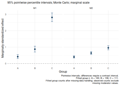
The default report includes each observed category. The continuous-moderator curve example above should not be interpreted as interpolating between groups.
Confidence intervals, bootstrap and both engines
Each valid joint draw supplies both regression coefficients and model-implied SDs. Transform the effect using those draw-specific SDs, then summarize the transformed draws. For continuous moderators, the selected raw values (for example the reference mean and mean plus/minus one reference SD) remain fixed across draws. If standardized coefficients are used, evaluate them at in draw , not at one fixed standardized moderator value.
Point estimates evaluate the effect at the fitted parameters, or at
pooled primitive parameters for MI. For MI models with products of
mediator differences and the moderator, the marginal variance estimators
are pooled jointly with those coefficients before taking square roots.
Point estimates are not averages of nonlinear draw effects. Invalid
joint draws are excluded together; use
wsmed_effects(result)$diagnostics to inspect the query
diagnostics.
The current effect reports from print(),
summary() and wsmed_effects(), and
confint() applied to extracted effects, use percentile
intervals for both MC and bootstrap, with or without
moderation. They use R’s type-7 quantiles.
boot_ci_type affects stored legacy parameter tables; it
does not change these effect intervals. See the expandable
implementation notes below for the legacy conventions.
The following longer bootstrap example is not run during vignette rebuilding:
both_result <- wsMed(
  data = dat,
  M_C1 = c("M11", "M21"),
  M_C2 = c("M12", "M22"),
  Y_C1 = "Y1",
  Y_C2 = "Y2",
  W = "W",
  MP = c("b1", "d1"),
  ci_method = "both",
  standardized = TRUE
)
print(both_result)
summary(
  both_result,
  method = "mc"
)
summary(
  both_result,
  method = "bootstrap"
)
plot(
  both_result,
  method = "bootstrap"
)
When both engines are stored, print() reports both. Use
method in summary() and plot() to
select one engine.
Missing data and reporting
FIML and MI use the same effect definition. With
fixed.x = FALSE, estimated external moments participate in
the joint transformation. With fixed.x = TRUE,
transformations condition on fitted external moments. Products
containing an endogenous mediator are modeled with auxiliary moment
equations and covariances with their upstream mediator disturbances.
This preserves the predictor moment structure when a reference group
changes. fixed.x applies to the remaining genuine exogenous
predictors; endogenous product moments are always estimated.
MI supports MC inference and evaluates effects at pooled primitive
parameters; its probing and centering reference is the first completed
dataset. With MI and fixed.x = TRUE, external moments from
that reference are held fixed. This does not introduce
population-relative moderator probing or a new imputation procedure.
For MI models with interactions involving mediator differences, wsMed averages each marginal variance estimate over completed datasets. It pools its covariance with the primitive coefficients using delta-method within-imputation covariances and Rubin’s rules. MC samples the variances jointly with the coefficients, so the denominator is not treated as fixed. Pooling the variance itself avoids the coding dependence of evaluating a nonlinear marginal variance only after pooling covariance-model parameters. This additional variance-pooling step is specific to those endogenous products; it is not applied to every MI model. Other models obtain marginal scales from the jointly drawn model parameters. The original coefficient pooling and imputation procedure are retained.
Report the condition difference direction, model and moderated paths,
moderator coding/reference and raw probe values, marginal SD definition,
missing-data method, fixed.x, inference engine, number of
valid draws and interval type. Distinguish standardized interaction
coefficients per SD of W from conditional indirect effects at particular
raw W values.
For serial and sparse models, see the custom-model tutorial. Their complete indirect effects follow the same endpoint scaling rule.
More plots for reporting
Start with plot(result) for the default display.
Optional named helpers include plot_effects() for an effect
forest, plot_conditional_effects() for group or
reference-level point intervals, and plot_contrasts() for
effect differences with their own confidence intervals. All three
support standardized and the MC/bootstrap
engine selection. See Plotting mediation effects and contrasts
for executed examples, selection of paths and labels, and export to PDF
or PNG.
Imputation compatibility
Correct standardization does not repair an imputation model that
omits substantive interactions. Default raw-variable MI uses main
effects. To use model-compatible external imputations, pass a list of
completed wide datasets (or a mice mids object) through
wsmed_fit(..., missing = "mi", mi = list(completed = completed))
or
wsMed(..., Na = "MI", mi_args = list(completed = completed)).
The difference scores and products are regenerated in each completion;
observed cells and factor levels are checked. See the worked example for assumptions,
an explicit SMC-FCS predictor matrix and convergence guidance.
Optional implementation checks
Expand numerical checks and legacy moderation-table details
These checks inspect stored internals. They are not required to
request standardized results through summary(),
wsmed_effects() or plot().
Check the stored point estimates
For this complete-data MC fit, the standardized overall effects must equal the raw effects divided by the fitted marginal outcome SD:
sy <- sqrt(lavaan::fitted(result$mc$fit)$cov["Ydiff", "Ydiff"])
stopifnot(isTRUE(all.equal(
  result$moderation_std$conditional_overall$Estimate,
  result$moderation$conditional_overall$Estimate / sy,
  tolerance = 1e-7
)))
stopifnot(identical(result$moderation_std$theta_curve$W_raw,
                    result$moderation$theta_curve$W_raw))
This identity concerns point estimates. It does not justify dividing raw confidence limits by the fitted SD.
Legacy moderation tables
summary(result, standardized = TRUE) is sufficient for
ordinary reporting. The older standardize_moderation()
helper uses the joint MC or bootstrap draws stored in a
wsMed object with a moderator. It returns the standardized
moderation list:
converted <- standardize_moderation(result)
stopifnot(isTRUE(all.equal(converted, result$moderation_std)))
result$moderation_std <- converted
attr(converted, "standardization")
#> $effect_scale
#> [1] "marginal model-implied endpoint scales; IE / SD(Ydiff)"
#>
#> $moderator_units
#> [1] "raw; fixed numerical probes; dummy coding unchanged"
#>
#> $mod_coeff_units
#> [1] "per SD of continuous W; per 0/1 dummy contrast"
#>
#> $interval
#> [1] "percentile"
#>
#> $engine
#> [1] "mc"
#>
#> $fixed.x
#> [1] FALSE
#>
#> $MI_reference
#> NULL
#>
#> $diagnostics
#> $diagnostics$requested
#> [1] 20000
#>
#> $diagnostics$valid
#> [1] 20000
#>
#> $diagnostics$invalid
#> [1] 0
#>
#> $diagnostics$invalid_indices
#> integer(0)
#>
#> $diagnostics$reasons
#> < table of extent 0 >
A result without the required stored draws cannot be converted by this helper.
In standardized legacy parameter tables, "bc" and
"bca.simple" apply bias correction with zero acceleration;
this is not a full BCa calculation. Their bootstrap p-values require at
least 1,000 valid replicates. That threshold does not define the
availability of percentile effect CIs in the current interface.