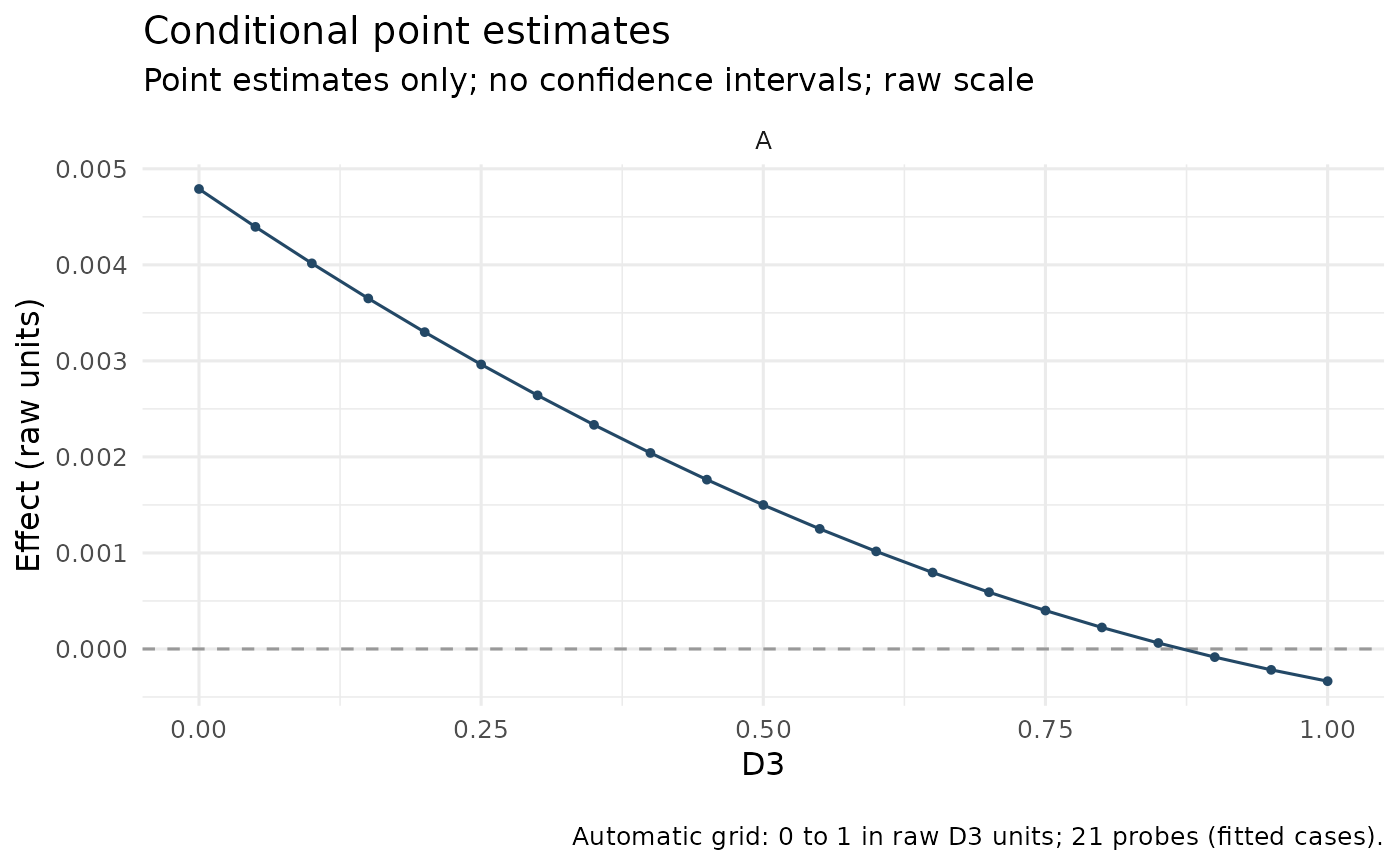
Plot stored effects without fitting, imputing, or drawing new samples.
The returned ggplot contains the full-precision plotted table in data.
Usage
# S3 method for class 'wsMed'
plot(
  x,
  type = "indirect",
  terms = NULL,
  at = NULL,
  scale = NULL,
  method = NULL,
  level = NULL,
  view = c("auto", "forest", "curve", "conditional"),
  n = 51L,
  labels = NULL,
  title = NULL,
  x_label = NULL,
  y_label = NULL,
  ncol = NULL,
  base_size = 12,
  rug = FALSE,
  standardized = NULL,
  ...
)

# S3 method for class 'wsmed_inference'
plot(
  x,
  type = "indirect",
  terms = NULL,
  at = NULL,
  scale = NULL,
  method = NULL,
  level = NULL,
  view = c("auto", "forest", "curve", "conditional"),
  n = 51L,
  labels = NULL,
  title = NULL,
  x_label = NULL,
  y_label = NULL,
  ncol = NULL,
  base_size = 12,
  rug = FALSE,
  standardized = NULL,
  ...
)

# S3 method for class 'wsmed_fit'
plot(
  x,
  type = "indirect",
  terms = NULL,
  at = NULL,
  scale = NULL,
  method = NULL,
  level = NULL,
  view = c("auto", "forest", "curve", "conditional"),
  n = 51L,
  labels = NULL,
  title = NULL,
  x_label = NULL,
  y_label = NULL,
  ncol = NULL,
  base_size = 12,
  rug = FALSE,
  standardized = NULL,
  ...
)

# S3 method for class 'wsmed_results'
plot(
  x,
  view = c("auto", "forest", "curve", "conditional"),
  terms = NULL,
  level = NULL,
  labels = NULL,
  title = NULL,
  x_label = NULL,
  y_label = NULL,
  ncol = NULL,
  base_size = 12,
  ...
)
Arguments
- x
A wsMed, wsmed_fit, wsmed_inference, or wsmed_results object.
- type
Effect family passed to
wsmed_effects().- terms
Effect identifiers to select, in display order. For a results object, use either effect identifiers or complete row identifiers.
- at
Named list of raw moderator values or factor labels.
- scale, method
Passed to
wsmed_effects(). Select method explicitly when a one-call object contains both Monte Carlo and bootstrap inference.- level
Confidence level. NULL retains the stored level. For an extracted results object, intervals can be recalculated from its stored effect draws.
- view
One of auto, forest, curve, or conditional. Auto uses a curve for a continuous moderator, separate category points for a categorical moderator, and a forest plot for unmoderated effects, single probes, and contrasts.
- n
Number of equally spaced probes for an automatic continuous curve (default 51). The range is the finite moderator range among cases used by the first fitted dataset. In MI this is the first completed dataset.
- labels
Named character vector mapping effect identifiers to labels. Labels must distinguish effects. Defaults use mediator role names.
- title, x_label, y_label
Optional title and axis labels.
- ncol
Number of facet columns, or NULL.
- base_size
Positive base font size.
- rug
Add observed raw moderator values along a continuous curve's horizontal axis. Available for fitted/inference/one-call objects only. Uses fitted cases with an observed moderator; imputed values are excluded.
- standardized
NULL inherits the analysis setting; TRUE or FALSE overrides it for this plot. Available on fit, inference and one-call objects.
- ...
Additional arguments are rejected to catch misspellings.
Value
A ggplot. Its wsmed_plot attribute records the method, scale,
confidence level, interval convention, view, and automatic-grid range.
Details
Curves connect finite probes; bands are pointwise percentile
intervals, not simultaneous bands or Johnson–Neyman regions. Supplied probes
outside the observed fitted-case range are identified in the caption and
plotted data (extrapolated). Group counts appear in categorical captions;
for MI these are ranges across completed datasets, not effective sample sizes.
Plot metadata retain support, including the observed range or group counts.
remain in raw units. A continuous conditional point plot requires explicit
at values. Forest plots without at use the usual reference value.
Category and effect selections retain their supplied order. A fitted object
without inference produces point estimates only, with no confidence band.
Extracted results contain only their selected effects and probes: plotting
them never invents a new grid. Use wsmed_effects() again to change the scale,
method, or probes. wsmed_contrasts() constructs differences from joint draws.
Marginal standardization uses the same draw-specific scales as effect
extraction; it does not standardize a plotted table after computing intervals.
The older plot_effects(), plot_conditional_effects(), plot_contrasts(),
and plot_moderation_curve() calls remain available. For wsMed objects those
helpers preserve the stored legacy tables, including requested bootstrap
interval types. The plot methods here use the percentile convention of
wsmed_effects(). Plots explicitly identify their interval source.